User guide

Input files

Configuration file

The file simulation.ini contains all the basic configurations to run a simulation.

Here are the different variables that you can configure:

Configuration name	Data type	Description
NB_PHOTONS	int	The number of photons used in the simulation
MAXIMUM_DEPTH	int	The maximum number of times that the light bounces in the scene
SCALE_FACTOR	int	The size of geometries. The vertices of geometries is recalculated by dividing their coordinates by this value
T_MIN	float	The minimum distance between the point of intersection and the origin of the light ray
NB_THREAD	int	The number of threads on the CPU used to calculate in parallel. This value is between 0 and the number of cores of your CPU.
BACKFACE_CULLING	yes/no	Define which mode of intersection is chosen: intersect only with the front face (yes) or intersect with both faces (no)
BASE_SPECTRAL_RANGE	int int	The base spectral range which includes all the other spectral ranges. The first value is the start of band and the second is the end of band. Ex: 100 200
DIVIDED_SPECTRAL_RANGE	int [int int]	The list of spectral ranges divided from the base spectral range. The first value is the number of divided parts, the value start and end of band is continue right after. These bands have to be smaller than the base spectral range. Ex: 2 100 150 150 200
RENDERING	0/1	1 for rendering an image after computation 0 for no image (faster)
KEEP_ALL	0/1	Whether or not to keep all the photons shot in a simulation. Can be useful to visualise what happened but very memory intensive. Use with caution
$ENVIRONMENT_FILE	string	The filepath of the environment to be loaded. Should be a rad file.
$OPTICAL_PROPERTIES_DIR	string	The path of the directory containing the optical properties of the objects.

This is an example of defining a configuration file.

$NB_PHOTONS 1000000000
$MAXIMUM_DEPTH 50
$SCALE_FACTOR 1
$T_MIN 0.1
$NB_THREAD 8
$BACKFACE_CULLING yes
$BASE_SPECTRAL_RANGE 400 800
$DIVIDED_SPECTRAL_RANGE 2 600 655 655 665

Room file

At this version, only files of type .rad is supported by our tool.

To define an object in a .rad file, there are two steps:

Firstly, we have to define the material object

void material_type material_name
0
0
material_data

Secondly, we will define an object with the name of a defined material and its geometries

Multiple objects can be defined from a single material

material_name geometry_type object_name
0
0
geometry_data

For each geometry_type and material_type, we will have the different ways to define the geometry_data and material_data

This is an example of a file .rad with the geometry type polygon and the material type metal

void metal Sol
0
0
5
0.37047683515999996 0.37047683515999996 0.37047683515999996 0.100 0

Sol polygon dallage
0
0
12
0.0 0.0 0
2400.0 0.0 0
2400.0 1840.0 0
0.0 1840.0 0

More information of the files .rad can be found in this file refman.pdf

Optical property files

The files containing the optical properties are saved in this structure of folder:

.

├── Specularities.xlsx

├── Env

│ ├── ReflectancesMean

│ │ ├── .csv files

│ ├── TransmittancesMean

│ │ ├── .csv files

├── Plant

│ ├── ReflectancesMean

│ │ ├── .csv files

│ ├── TransmittancesMean

│ │ ├── .csv files

The file Specularities.xlsx is used to define the specularities of the materials. These values represent the average specularities for all the wavelength.

Here is an example of this file

Material	Visually estimated value
Aquanappe	0.1
CentrePlafond	0.5
CorniereAlu	0.3
PiedsTablette	0.3
MiroirCaissonLampes	0.4

The folder Env contains the files .csv which define the average reflection and average transmission for each wavelength of the environment’s objects.

These objects are rarely changing during the process of experiment.

Whereas, the files .csv inside the folder Plant is using to define these optical properties of sensor/plant.

The amount of received energies is calculated on these objects.

It is important to notice that the name of the .csv files is the same as the name of material which is defined in the room file (.rad)

For example:

lambda	moy
300	0.126
301	0.135
302	0.145
…	…

Sensor file

In our tool, we have a csv file defining the position and orientation of each sensor.

It goes as follows:

X	Y	Z	rayon_capteur	Xnorm	Ynorm	Znorm
110	930	1000	10	0	0	1
210	930	1000	10	0	0	1
310	930	1000	10	0	0	1
…	…	…	…	…	…	…

Plant file

To add a plant to the simulation, we use the Lpy to define the structure of a plant.

More information can be found in this link https://lpy.readthedocs.io/en/latest/index.html

Spectral heterogeneity file

The spectral heterogeneity file contains the information of the heterogeneity of the spectrum. In this file, there are the values of energies calculated en umol/m²/s which represent the flow of photons on each wavelength

This is an example of this file

wavelength(nm)	measured PPFD (umol m-2 s-1 nm-1)
401	0.0555
403	0.086
405	0.14
…	…

Calibration points file

The calibration points file contains the sensors which is used to convert the results from a number of photons to irradiance. This function only work for the simulation with sensors.

This is an example of this file

X	Y	Z	Nmes_start1_end1	Nmes_start2_end2	…	Nmes_startn_endn
610	1330	1400	3.91336	19.6182	…	value_1
710	1330	1400	4.17343	20.8869	…	value_2
1210	1330	1400	3.80179	18.8231	…	value_3
…	…	…	…	…	…	…

Run a simple simulation

These are the basic steps to run a simple light simulation with this tool:

Setup input files

Create a configuration file (simulation.ini)

$NB_PHOTONS 1000000000
$MAXIMUM_DEPTH 50
$SCALE_FACTOR 1
$T_MIN 0.1
$NB_THREAD 8
$BACKFACE_CULLING yes
$BASE_SPECTRAL_RANGE 400 800
$DIVIDED_SPECTRAL_RANGE 2 600 655 655 665

Create a room file (testChamber.rad) with only one light

void light lum400
0
0
3
0.4 0.4 0.4

lum400 cylinder lamp
0
0
7
715.62 1670.0 2105.0
743.193 1670.0 2105.0
0.1

Create a sensor file (captors_expe1.csv) with only one sensor

X,Y,Z,rayon_capteur,Xnorm,Ynorm,Znorm
110,930,1000,10,0,0,1

Create a folder ./PO to save the optical property of all the object. To simplify, we can leave it empty for now.

The calibration points file and spectral heterogeneity file are optional.

Write the core program

Create a python file (main.py) which contains the core program

from openalea.spice.simulator import Simulator

if __name__ == "__main__":

    simulator = Simulator(config_file="simulation.ini")
    simulator.addVirtualDiskSensorsFromFile("sensors_expe1.csv")
    simulator.run()
    simulator.results.writeResults() #write results to a file

Run and results

To run the program, you need to install the tools by following this guide.

Activate the conda environment and run the program.

mamba activate env_name
python main.py

The result is a csv file saved in the folder ./result. This is an example of result.

id	N_sim_600_655	N_sim_655_665
0	13635	13966

Calibrate the results

After running the simulation, we will obtain a result with the number of photons received on each sensors or organs of plant. But in reality, to using this result to do the further researches, we have to convert the unit of the current result to a unit which is more physical.

To do that, after finishing the simulation, we will do the calibration the result by using the function calibrateResults.

calibrated_res = simulator.calibrateResults("spectrum/chambre1_spectrum", "points_calibration.csv")
calibrated_res.writeResults() #write results to a file

To making this function works properly, we need two input files: the spectral heterogeneity file and the calibration points file.

In our tool, for each simulation of each spectral range, we will always run the same simulation of photon mapping. So the result final isn’t include the factor of spectral heterogeneity. That is why we need the spectral heterogeneity file to correct the final results of simulation before doing the calculations before that.

After correcting the factor of heterogeneity, we will calibrate the result by using the calibration point file. This file contains the received energies measured in reality on the positions of some sensors which is used in the simulation. With these values, we will use the method Linear Regression to calculate the coefficients to convert the results of simulation to irradiance (a unit used to measure the power of energy).

This function is only working with the simulation of sensors.

Visualize the room

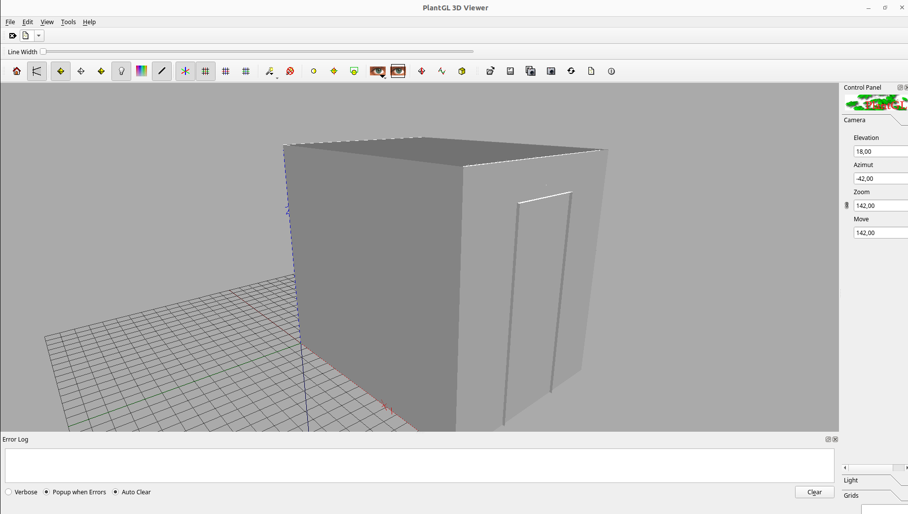
To visualize the room, after defining the input files, we use a function named visualizeScene. Here is the complete code for this program:

from openalea.spice.simulator import Simulator

if __name__ == "__main__":

    simulator = Simulator(config_file="simulation.ini")
    simulator.addVirtualDiskSensorsFromFile("sensors_expe1.csv")
    simulator.visualizeScene("ipython")

To obtain the 3D scene, we have to run this program through ipython or if in a notebook we use oawidgets.

ipython
%gui qt5
run main.py

Here is the plantGL interface to visualize the scene

It is also possible to visualize the simulation’s results in different ways with two other functions:

• visualizeResults which will apply a color map on each sensor object depending on the number of photons on it. By default the colormap used is ‘jet’.

• visualizePhotons which will display all the photons in the photon map in a 3d scene.

Warning

The function visualizePhotons will create each individual photons in the scene. This can be very intensive. Use with caution.

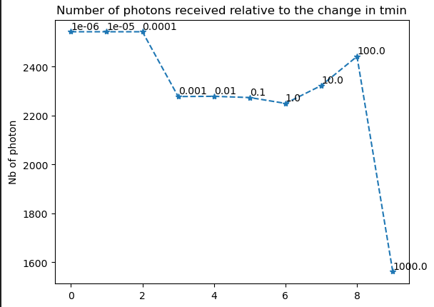
Test value Tmin

While running the simulation, we risk encountering the problem of auto-intersection if the value of Tmin is too small.

To avoid this problem, we’ve created a function to run the simulation with different values of Tmin. The result of this function is a graph showing the change in the number of photons after testing different values of Tmin.

Here is the complete code for this program:

from openalea.spice.simulator import Simulator

if __name__ == "__main__":

    simulator = Simulator(config_file="simulation.ini")
    simulator.addVirtualDiskSensorsFromFile("sensors_expe1.csv")
    simulator.test_t_min(int(1e6), 1e-6, 10, True)

Here is a example of result

We can find out the suitable range of value Tmin by finding the range where the result is the most stable (not changing). In this graph above, we can see that when the value tmin is between 0.001 and 100, our simulation doesn’t encountering the problem of auto-intersection.